Plot Vectors

Plotting vectors is handled by pygmt.Figure.plot.

Note

This tutorial assumes the use of a Python notebook, such as IPython or Jupyter Notebook. To see the figures while using a Python script instead, use fig.show(method="external") to display the figure in the default PDF viewer.

To save the figure, use fig.savefig("figname.pdf") where "figname.pdf" is the desired name and file extension for the saved figure.

# TODO: change this number to reflect the correct thumbnail

import numpy as np
import pygmt

"""
# Plot Vectors
----------

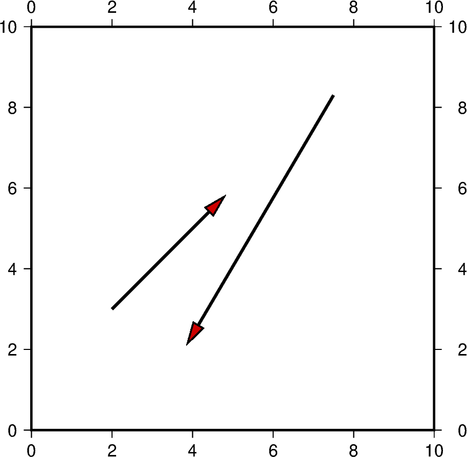
Create a Cartesian figure using ``projection`` parameter and set the axis scales
using ``region`` (in this case, each axis is 0-25). Pass a ``numpy`` array object that contains lists of all the vectors to be plotted.
"""
# vector specifications structured as: [x_start, y_start, direction_degrees, magnitude]
vector_1 = [2, 3, 45, 4]
vector_2 = [7.5, 8.3, -120.5, 7.2]
# Create a list of lists that include each vector information
data = np.array([vector_1] + [vector_2])

fig = pygmt.Figure()
fig.plot(
    region=[0, 10, 0, 10],
    projection="X10c/10c",
    frame="a",
    data=data,
    style="v0.6c+e",
    pen="2p",
    color="red3",
)
fig.show()

Out:

<IPython.core.display.Image object>

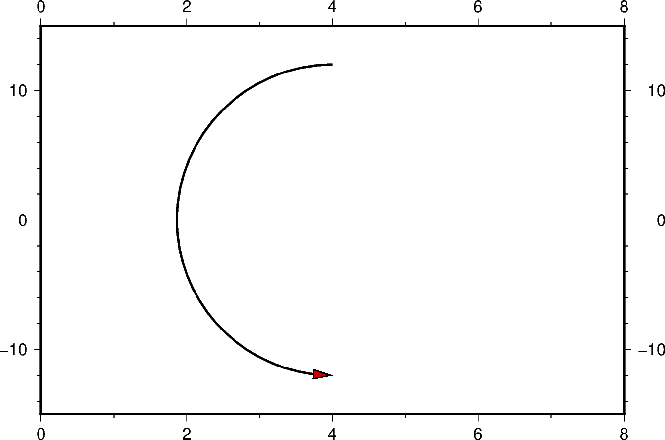
Circular vectors can be plotted using an x and y value to specify where the origin of the arc will be located on the plane. The variable diam is used to specify the diameter of the arc while the startDeg and stopDeg specify at what angle the arc will originate and end respectively.

fig = pygmt.Figure()

reg_x_lowbound = 0
reg_x_upperbound = 8
reg_y_lowbound = -15
reg_y_upperbound = 15

fig.basemap(
    region=[reg_x_lowbound, reg_x_upperbound, reg_y_lowbound, reg_y_upperbound],
    projection="X15c/10c",
    frame=True,
)

x = 4
y = 0
diam = 4
startDeg = 90
stopDeg = 270

data = np.array([[x, y, diam, startDeg, stopDeg]])
fig.plot(data=data, style="m0.5c+ea", color="red3", pen="1.5p,black")
fig.show()

Out:

<IPython.core.display.Image object>

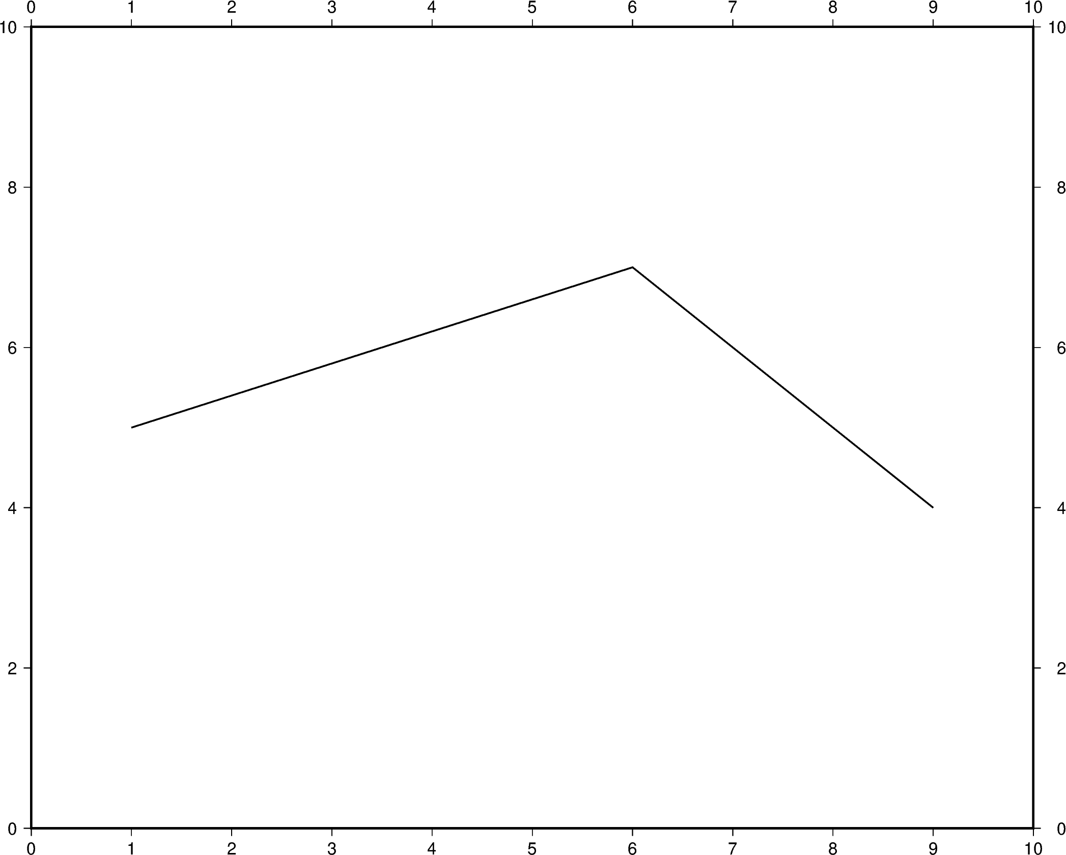
Additional line segments can be added by including additional values for x and y.

fig = pygmt.Figure()
fig.plot(
    region=[0, 10, 0, 10],
    projection="X25c/20c",
    frame="a",
    x=[1, 6, 9],
    y=[5, 7, 4],
    pen="1p,black",
)
fig.show()

Out:

<IPython.core.display.Image object>

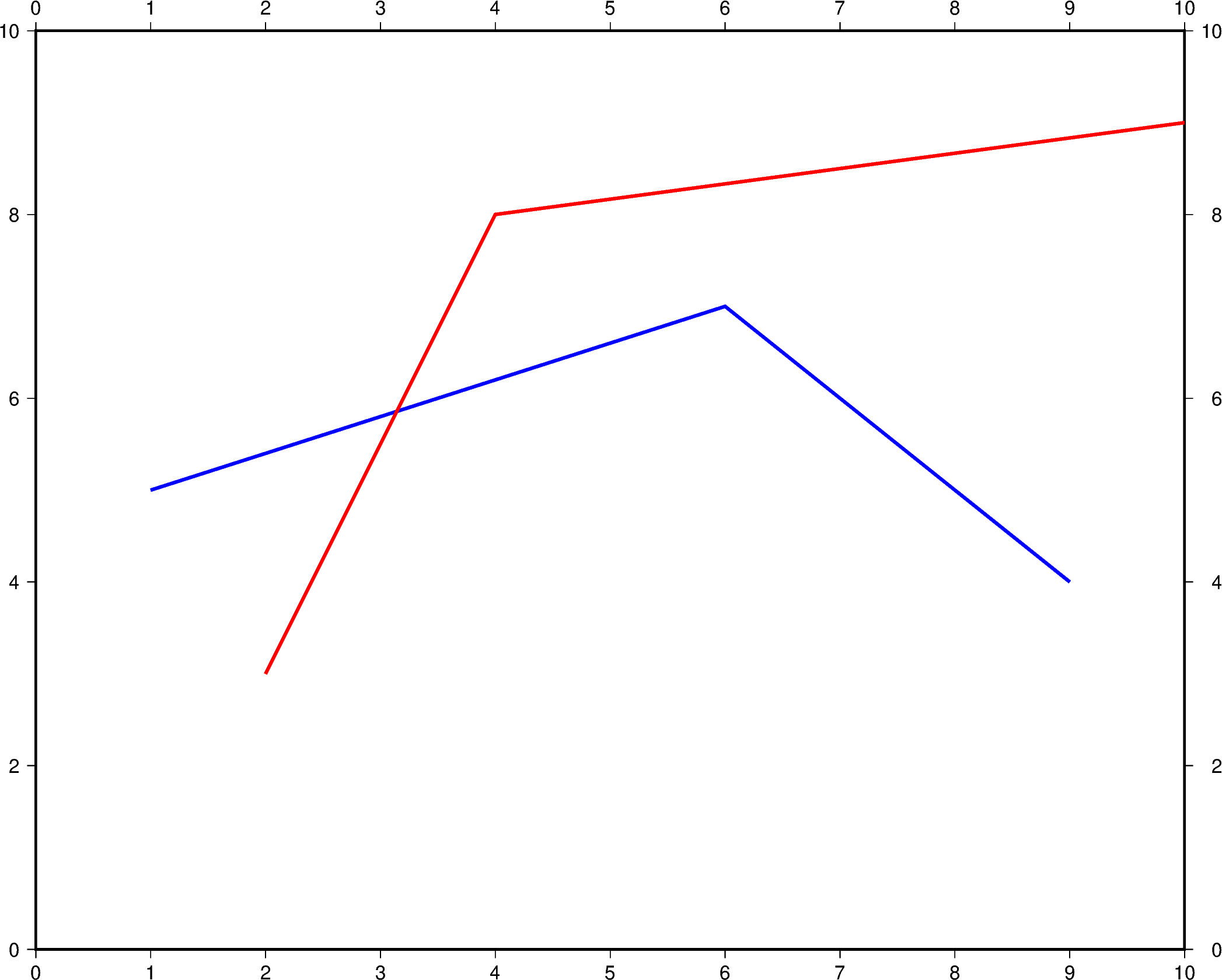
To plot multiple lines, pygmt.Figure.plot needs to be used for each additional line. Arguments such as region, projection, and frame do not need to be repeated in subsequent uses.

fig = pygmt.Figure()
fig.plot(
    region=[0, 10, 0, 10],
    projection="X25c/20c",
    frame="a",
    x=[1, 6, 9],
    y=[5, 7, 4],
    pen="2p,blue",
)
fig.plot(x=[2, 4, 10], y=[3, 8, 9], pen="2p,red")
fig.show()

Out:

<IPython.core.display.Image object>

Change line attributes

The line attributes can be set by the pen parameter. pen takes a string argument with the optional values width,color,style.

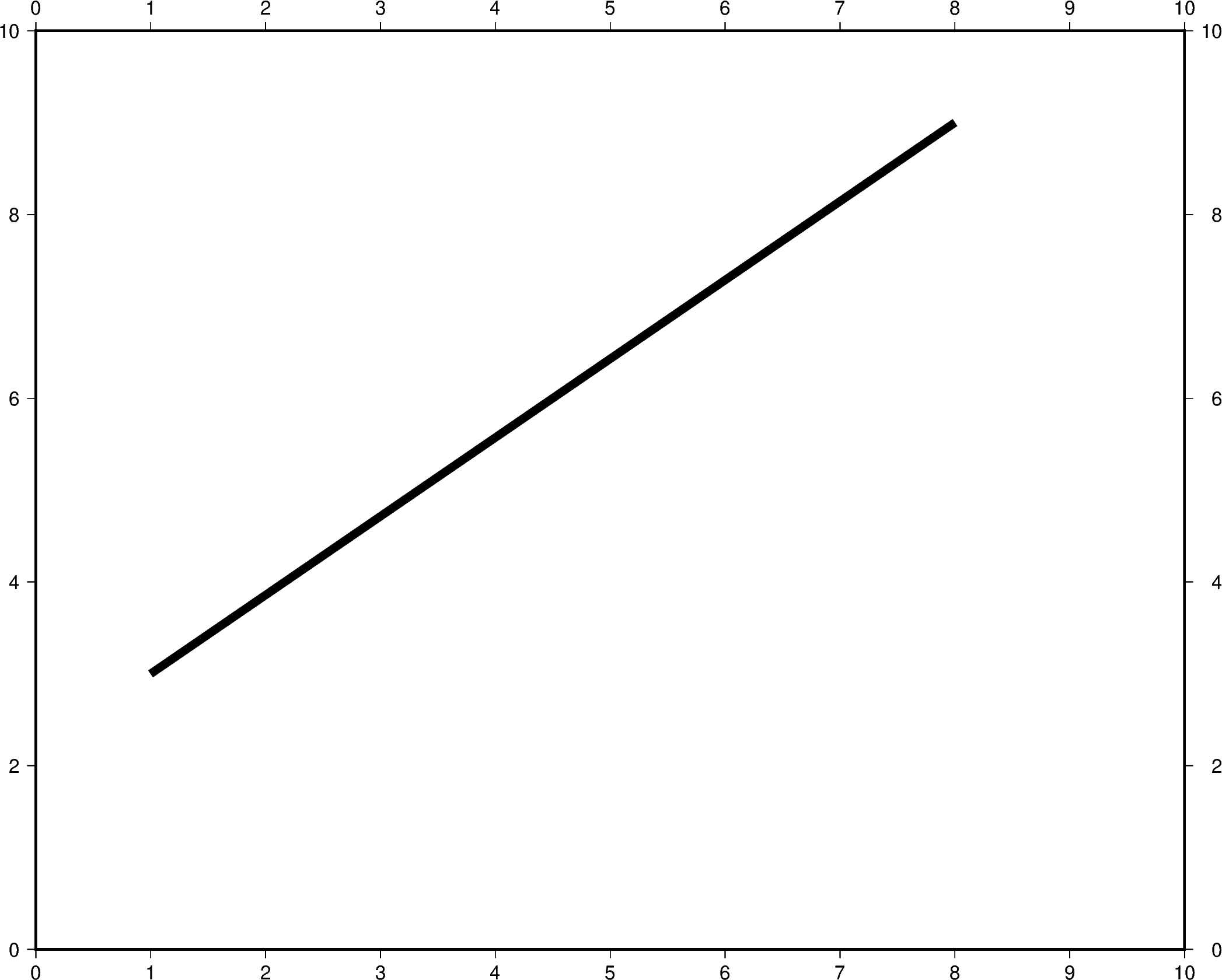
In the example below, the pen width is set to 5p, and with black as the default color and solid as the default style.

fig = pygmt.Figure()
fig.plot(
    region=[0, 10, 0, 10],
    projection="X25c/20c",
    frame="a",
    x=[1, 8],
    y=[3, 9],
    pen="5p",
)
fig.show()

Out:

<IPython.core.display.Image object>

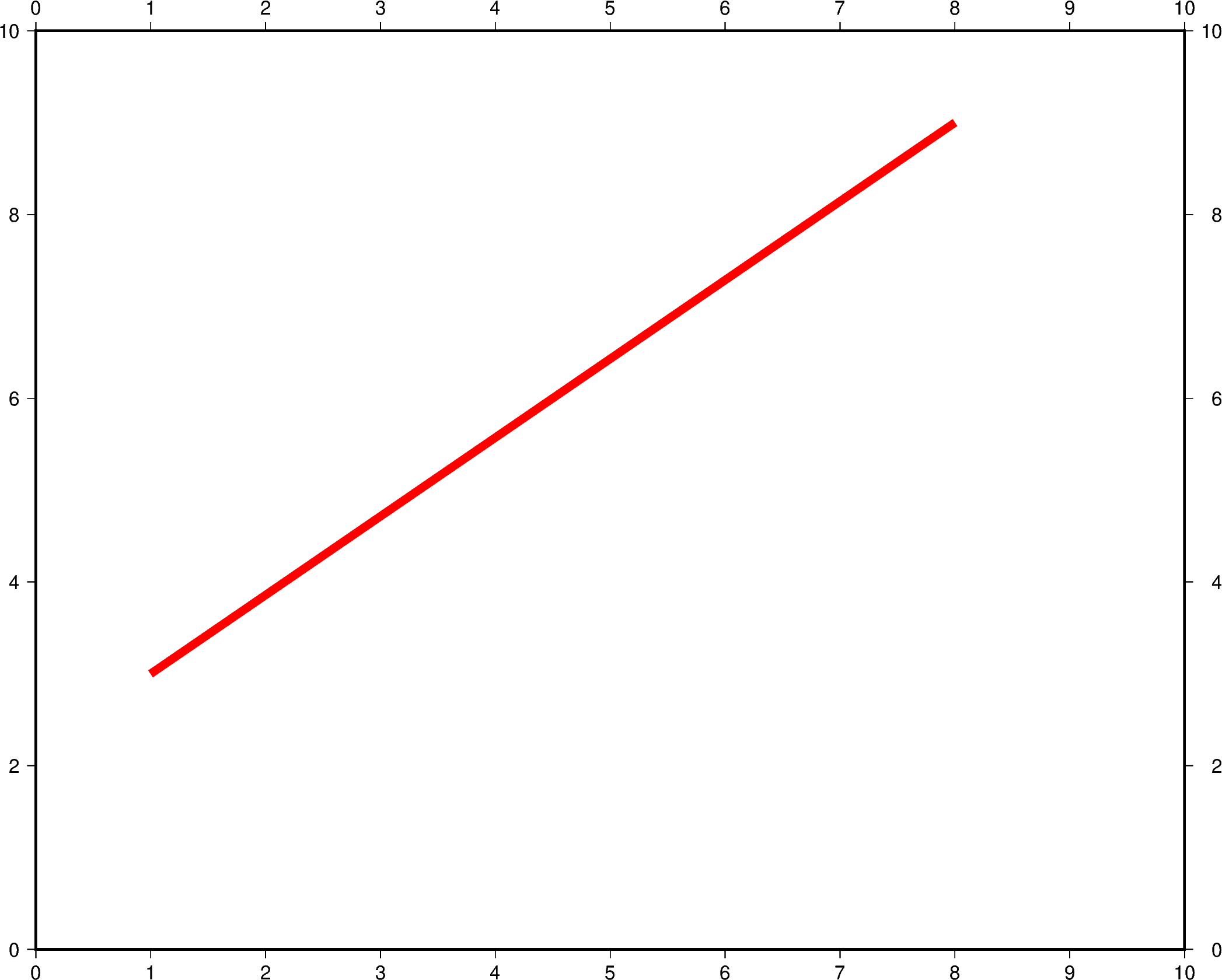
The line color can be set and is added after the line width to the pen parameter. In the example below, the line color is set to red.

fig = pygmt.Figure()
fig.plot(
    region=[0, 10, 0, 10],
    projection="X25c/20c",
    frame="a",
    x=[1, 8],
    y=[3, 9],
    pen="5p,red",
)
fig.show()

Out:

<IPython.core.display.Image object>

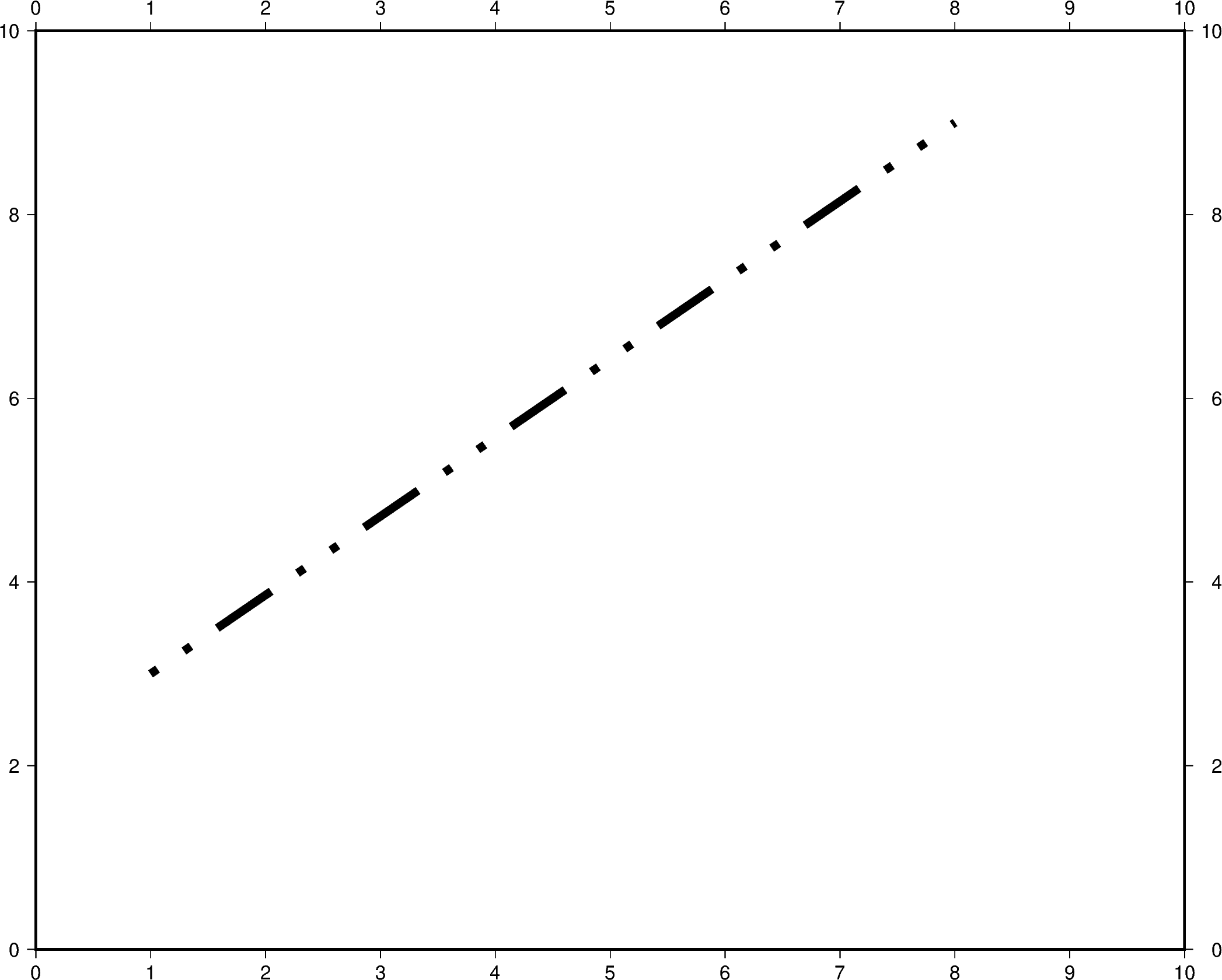
The line style can be set and is added after the line width or color to the pen parameter. In the example below, the line style is set to ..- (dot dot dash), and the default color black is used.

fig = pygmt.Figure()
fig.plot(
    region=[0, 10, 0, 10],
    projection="X25c/20c",
    frame="a",
    x=[1, 8],
    y=[3, 9],
    pen="5p,..-",
)
fig.show()

Out:

<IPython.core.display.Image object>

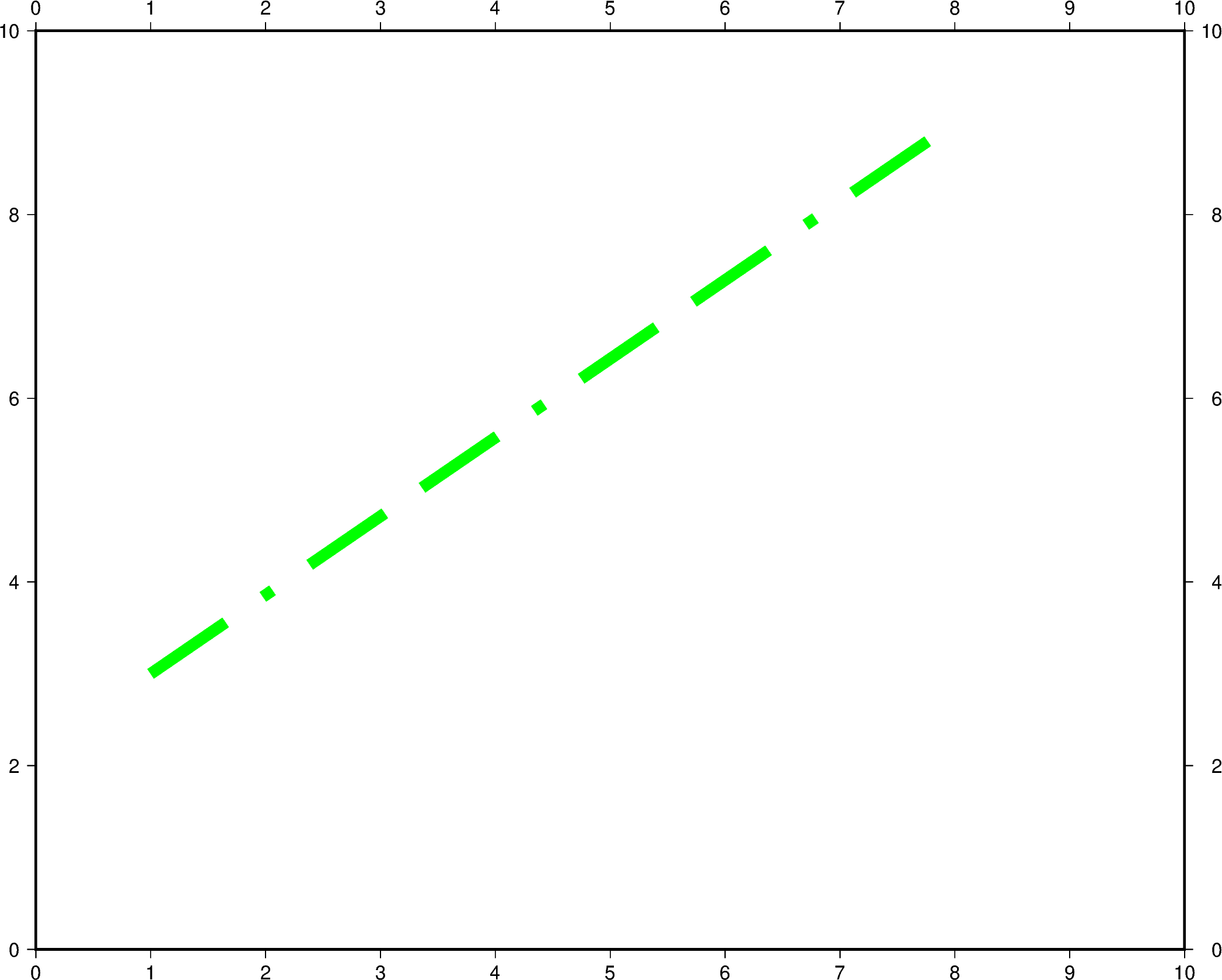
The line width, color, and style can all be set in the same pen parameter. In the example below, the line width is set to 7p, the color is set to green, and the line style is -.- (dash dot dash).

For a gallery showing other pen settings, see Line styles.

fig = pygmt.Figure()
fig.plot(
    region=[0, 10, 0, 10],
    projection="X25c/20c",
    frame="a",
    x=[1, 8],
    y=[3, 9],
    pen="7p,green,-.-",
)
fig.show()

Out:

<IPython.core.display.Image object>